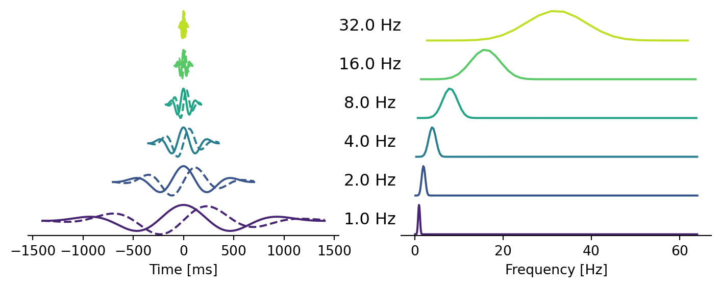
import matplotlib.pyplot as plt
from meeglet import define_frequencies, define_wavelets, plot_wavelet_family
= define_frequencies(
foi, sigma_time, sigma_freq, bw_oct, qt =1, foi_end=32, bw_oct=1, delta_oct=1
foi_start
)
= define_wavelets(
wavelets =foi, sigma_time=sigma_time, sfreq=1000., density='oct'
foi
)
=64)
plot_wavelet_family(wavelets, foi, fmax9, 3) plt.gcf().set_size_inches(
Machine learning of brain-specific biomarkers from EEG
Our work on machine-learning for EEG biomarkers in eBioMedicine!
To preprocess or not to preprocess your #EEG (when using #ML models for building 🧠🧑🔬 #brain #biomarkers)🔮?
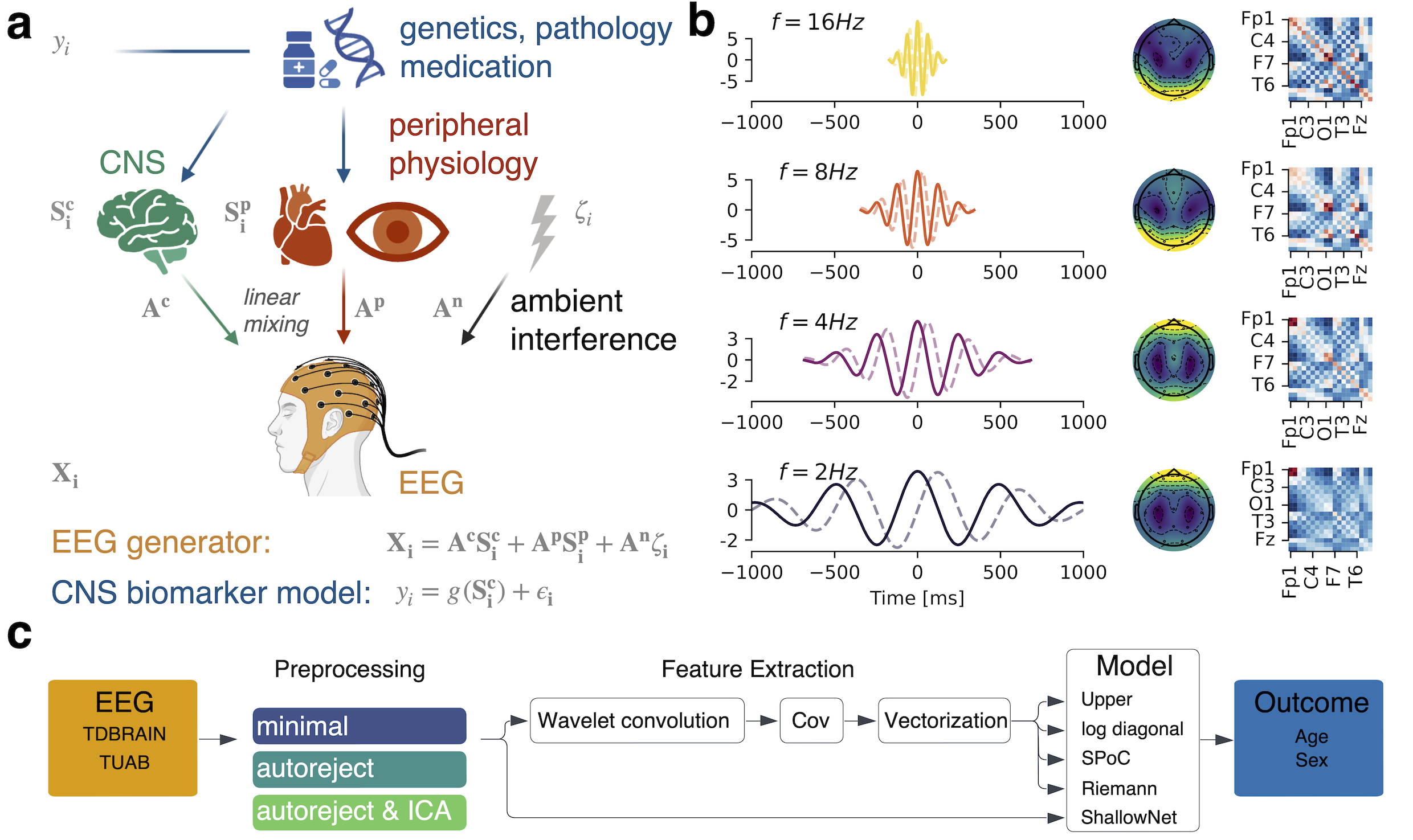
The impact of artifact handling on #ML models for #EEG is often neglected — see e.g. the brilliant review by (Roy et al. 2019). Importantly, in biomarker applications of EEG, genetics, medical conditions or medication not only affect the brain but also different body systems, leading to consequential signal mixing (Figure 1 a). Previous work on predictive regression modeling (D. Sabbagh et al. 2019; David Sabbagh et al. 2020) has a term for noise but does not handle predictive non-brain signals. Here we extended the generative model and thereby convinced ourselves that without precautions, #ML models will pick up whatever predictive signal is found – whether from the brain or the body.
Note that figure numbering deviates in this document from the paper, hence, where needed, the original figure number in parentheses in figure captions.
Problem and approach
Can we find evidence for contamination of ML models for EEG by predictive artifacts generated by body signals or even quantify it? In this work, we upgraded the previous covariance-based pipelines to use Morlet Wavelets as in (Hipp et al. 2012). This enabled head-to-head comparisons between well-established EEG biomarker methods focusing on the log-power spectrum (Frohlich et al. 2019b, 2019a, 2019c; Hawellek et al. 2022; Hipp, Knoflach, et al. 2021; Forsyth et al. 2018; Hipp, Frohlich, et al. 2021) and #ML models based on covariance matrices (David Sabbagh et al. 2020) as representations (Figure 1 b). We then got inspired to systematically explore the impact of #EEG artifact removal on different covariance-based models as well as a simple artificial neural network – the ShallowNet by (Schirrmeister et al. 2017) on two large datasets, TDBRAIN and TUAB for 2 model tasks, i.e., age- and sex-prediction (Figure 1 b). Moreover, we developed several practical sensitivity analyses to gauge the extent of signal mixing in predictive models to help identify the brain-specific information captured by the model (more on that below).
Basic denoising improves model performance, artifact-removal reduces model performance
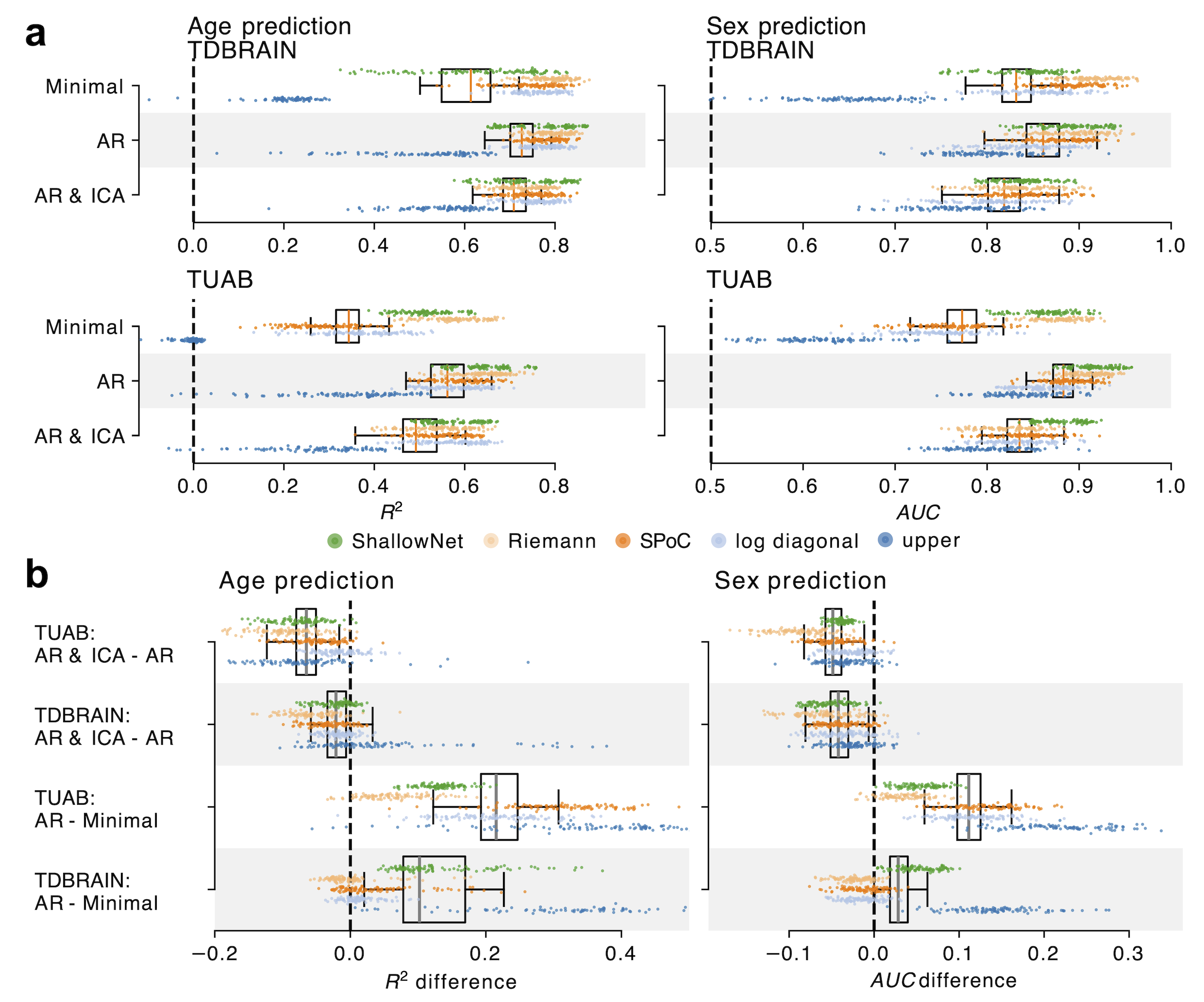
Comparing the impact of basic denoising via Autoreject VS ICA-based cleaning of bodily artifacts on the prediction performance of the classical covariance-based models from (David Sabbagh et al. 2020) and the ShallowNet (Schirrmeister et al. 2017) revealed a striking pattern (Figure 2). Some denoising improves model performance (especially for weak models) whereas ICA-based cleaning can hurt performance! What is behind that? Are those artifact components removed by ICA predictive?
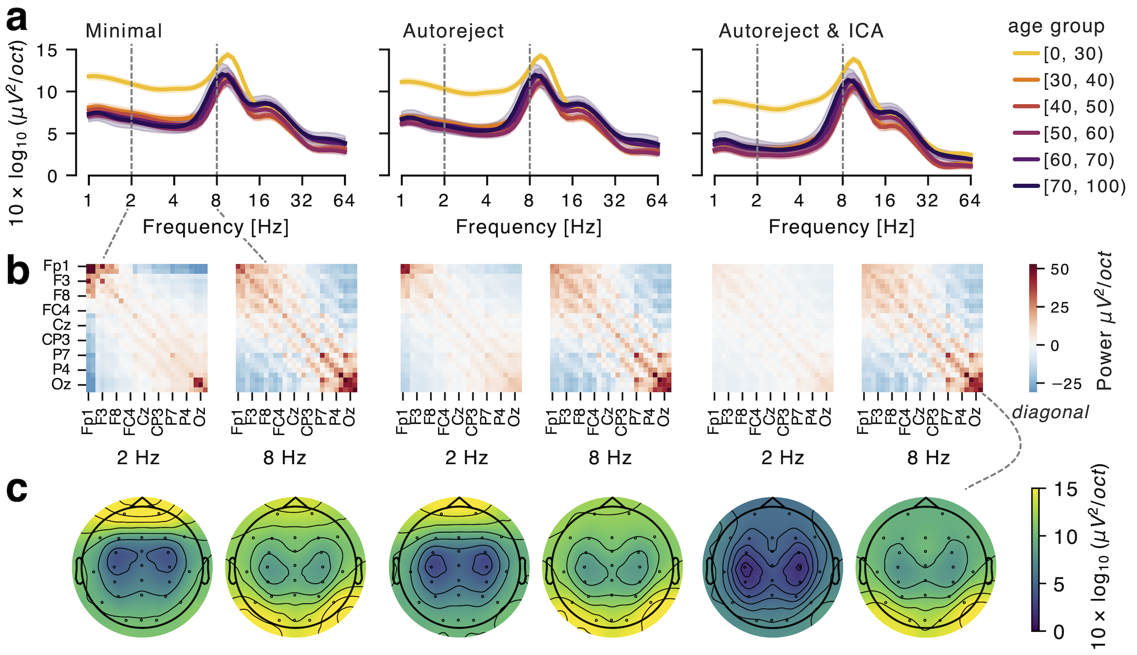
Deep dive via Figure 3. Just to be sure, Autoreject does not remove eye blinks whereas ICA does. This is seen most clearly on covariances and power topographies around 2Hz. So what is going on here? (Btw. an example of how our Morlet Wavelet approach allowed us to read out and compare different popular EEG descriptors for the same wavelets at the same frequencies).
Estimating to the degree to which ML models listen to brain signals VS body signals
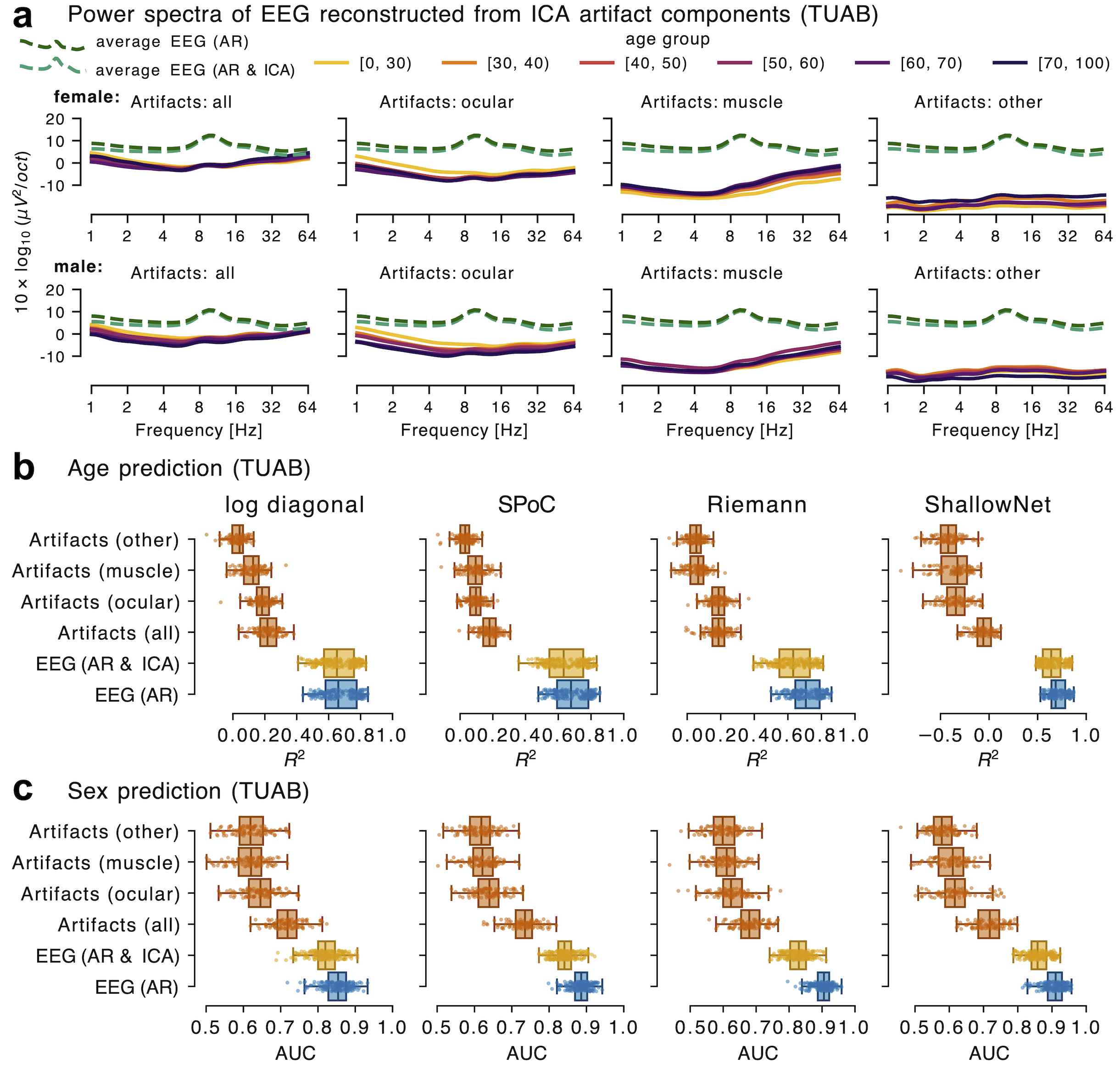
One way to figure out if artifacts are predictive is using ICA to isolate non-brain sources and reconstruct the same EEG features from that subspace. We see that artifact components show some co-variation with age and sex (Figure 4). As hypothesized, sex- and age-prediction is possible from those components. Calmingly, the performance for clean EEG is higher than for those artifact-derived EEG signals. Btw. if you are into stats, checkout our theoretical expansion of the Sabbagh et al. generative model that we used to motivate this analysis, eqs. 1-3 & 14-15 in the paper.
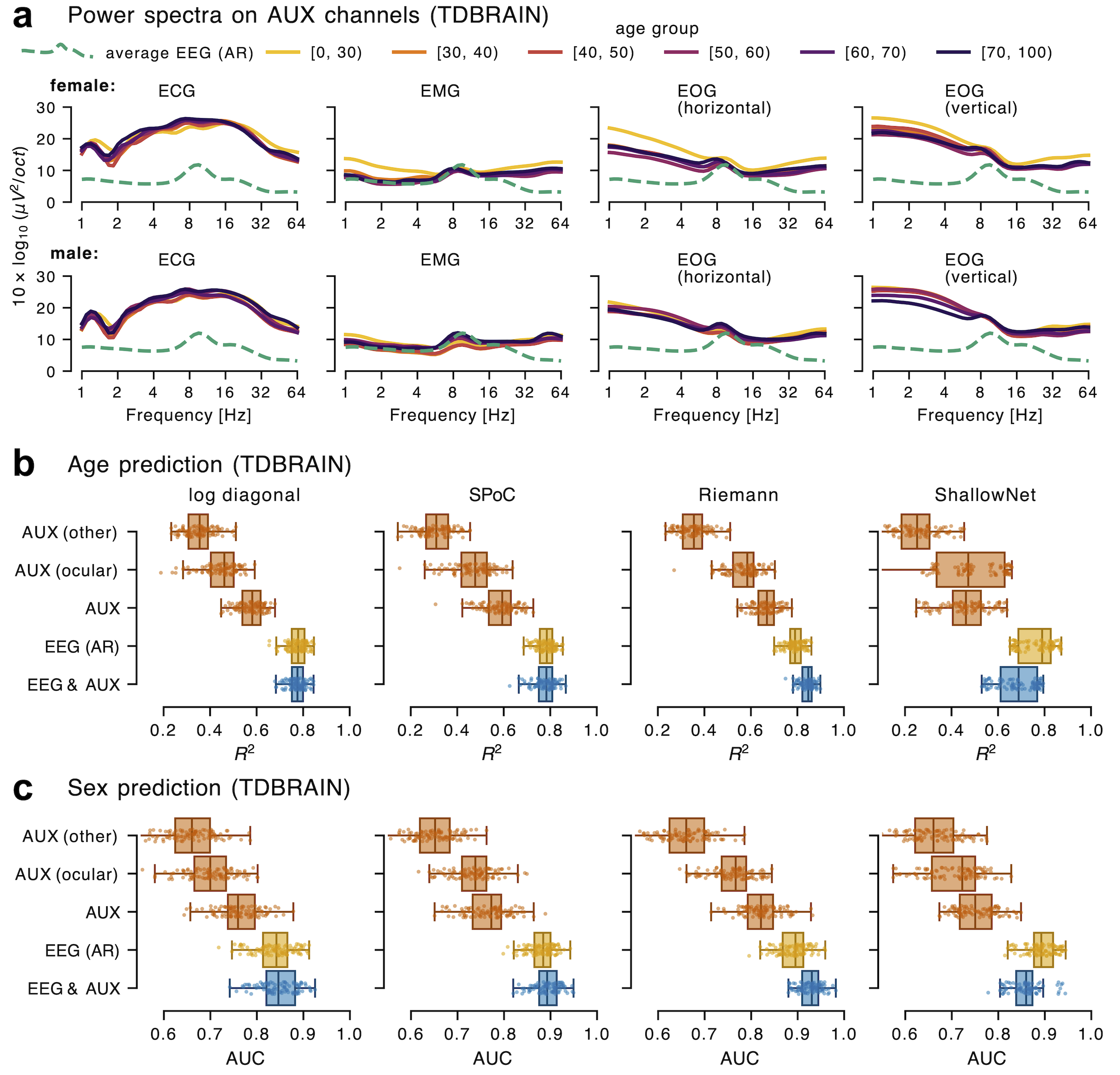
If you have auxiliary channels (EMG, EOG, ECG, etc.), as was the case with the highly controlled EEG recordings from the TDBRAIN dataset, another route for probing this point is doing a same-analysis sort of approach – as in (Görgen et al. 2018)– by computing the same EEG features from those AUX channels (Figure 5). A similar story unfolds, pointing at predictive information in AUX channels, in particular EOG. Ok now you might think that what we see here is some imperfect subspace estimation, leading to residual brain signals on AUX channels or in ICA components. This cannot be entirely excluded but on the other hand, we have prior knowledge about body-signal changes in different medical conditions leading to changes in artifact load. A careful view would, hence, be to see these estimates here as some form of upper bound.
We can regardless dig deeper and work harder to isolate specific artifacts (thank you unknown reviewers for motivating us!). Here we used the EOG channels in TDBRAIN to extract eye-blink times. We then use evoked-response methodology to suppress the non-timelocked background brain activity (Figure 6). We can then plug the EEG topographies at the maximum (which is the even time) into a linear decoder. To look behind trivial effects of blink-frequency, we repeat our analysis across subsamples of numbers of eye blinks and what we see remains the same: The spatial electrical propagation patterns induced by eye blinks are predictive of age and sex. (And the performance values fall within the upper bound provided by the previous analyses.)
Model inspection and exploration via spectral profiling
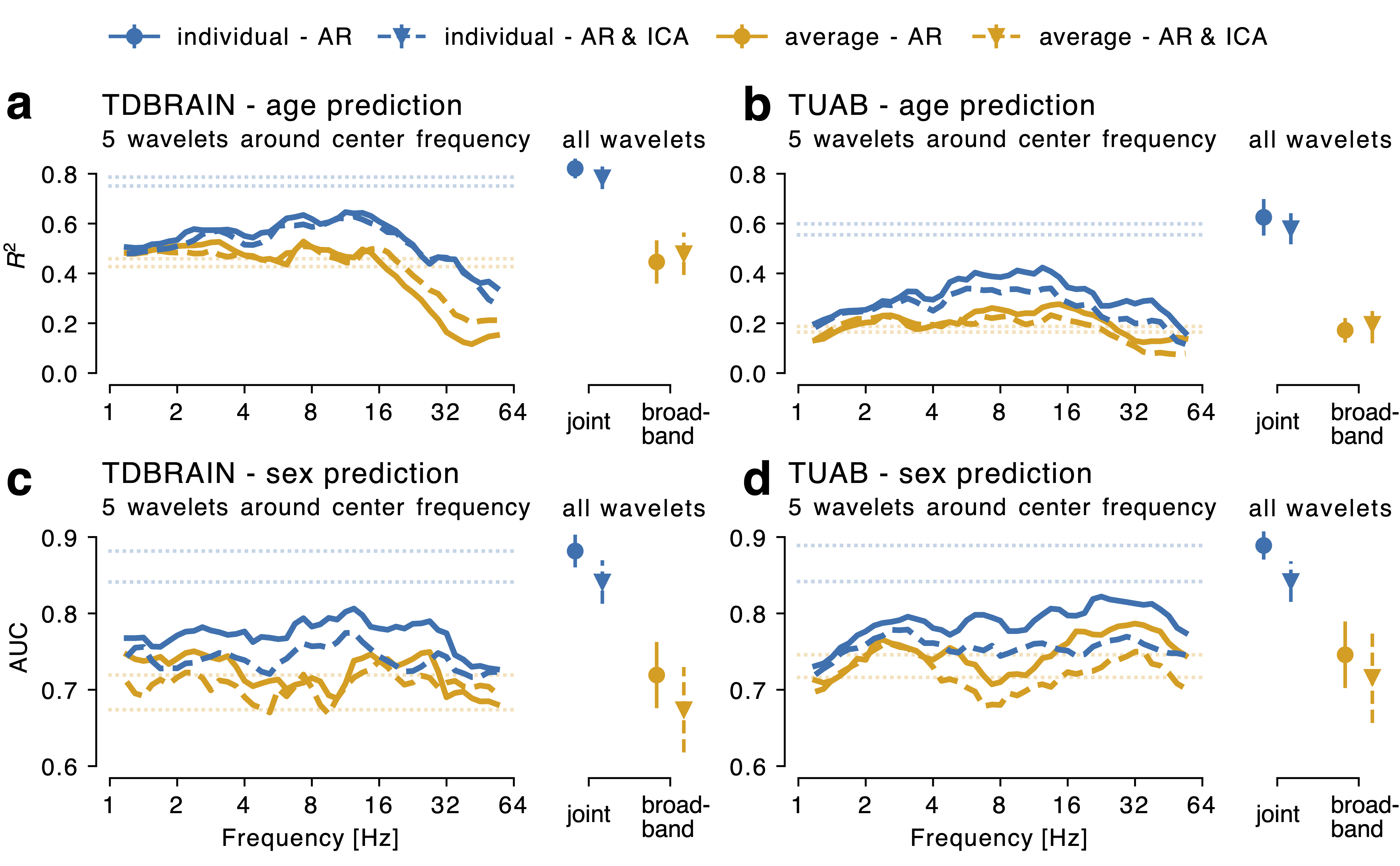
Time for looking at what else the tools powering our study can offer to support exploration. Here we benefit from the high-resolution grid of wavelets to explore the spectral specificity of our covariance-based prediction models (Figure 7). We can do that frequency-wise (individual, blue, left subplots) or pooling over 5 neighboring frequencies e.g. for picking up predictive edge effects (average, orange, left subplots). Across tasks and datasets, using multiple neighboring frequencies adds information. However, we can rule trivial broadband effects (right hand, orange, average) as performance degrades substantially when averaging over frequencies. Moreover, combining all frequencies led to the best performance (right hand, blue, individual). While some information is concentrated between 4-16Hz, these results suggest that information is widely distributed for these tasks and may contain not only oscillatory information coming from brain-rhythms but also anatomical information revealed by the spatial patterns resulting from electrical propagation. On this point, check out the excellent study by (Jochmann et al. 2023).
Morlet wavelets enhance model performance
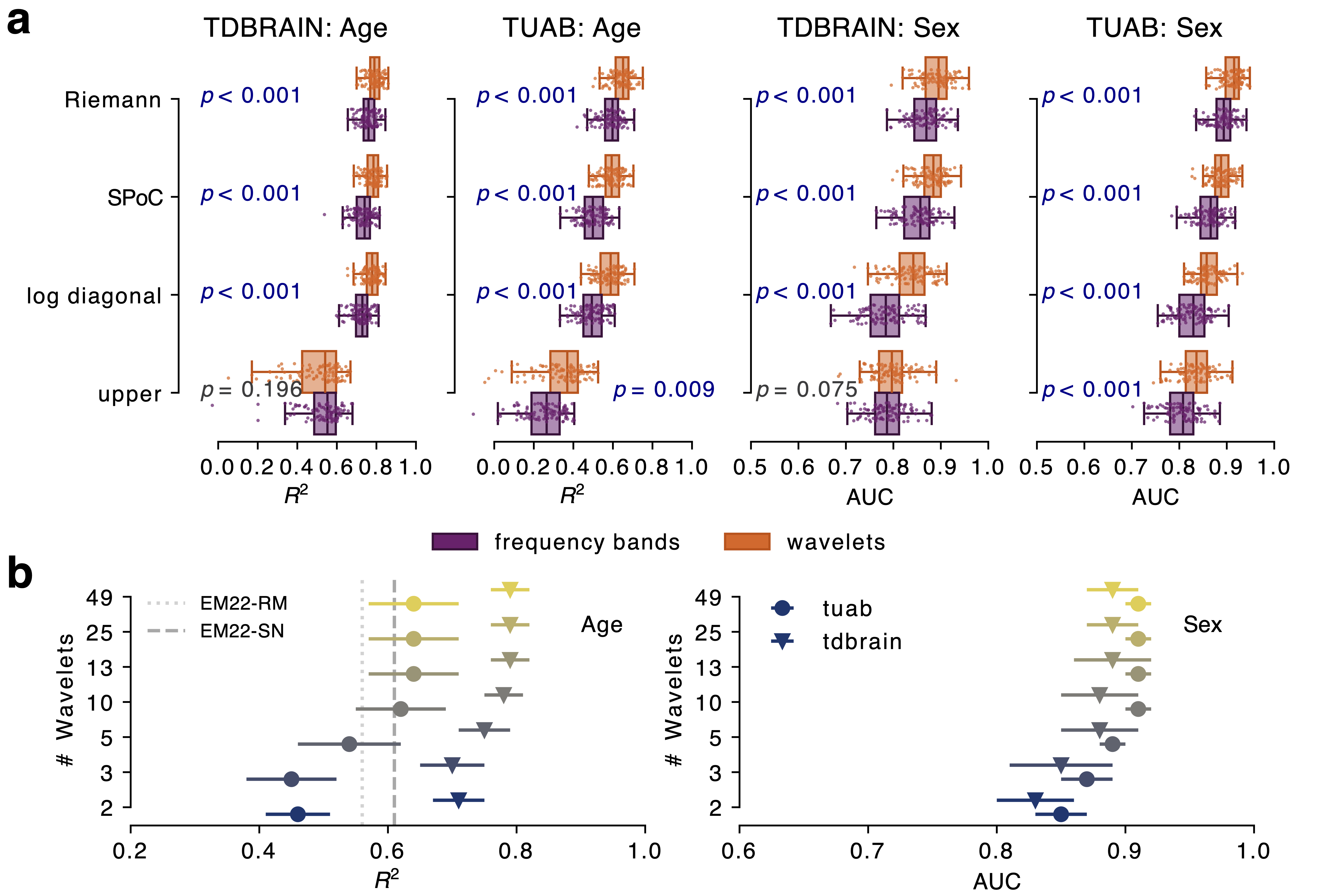
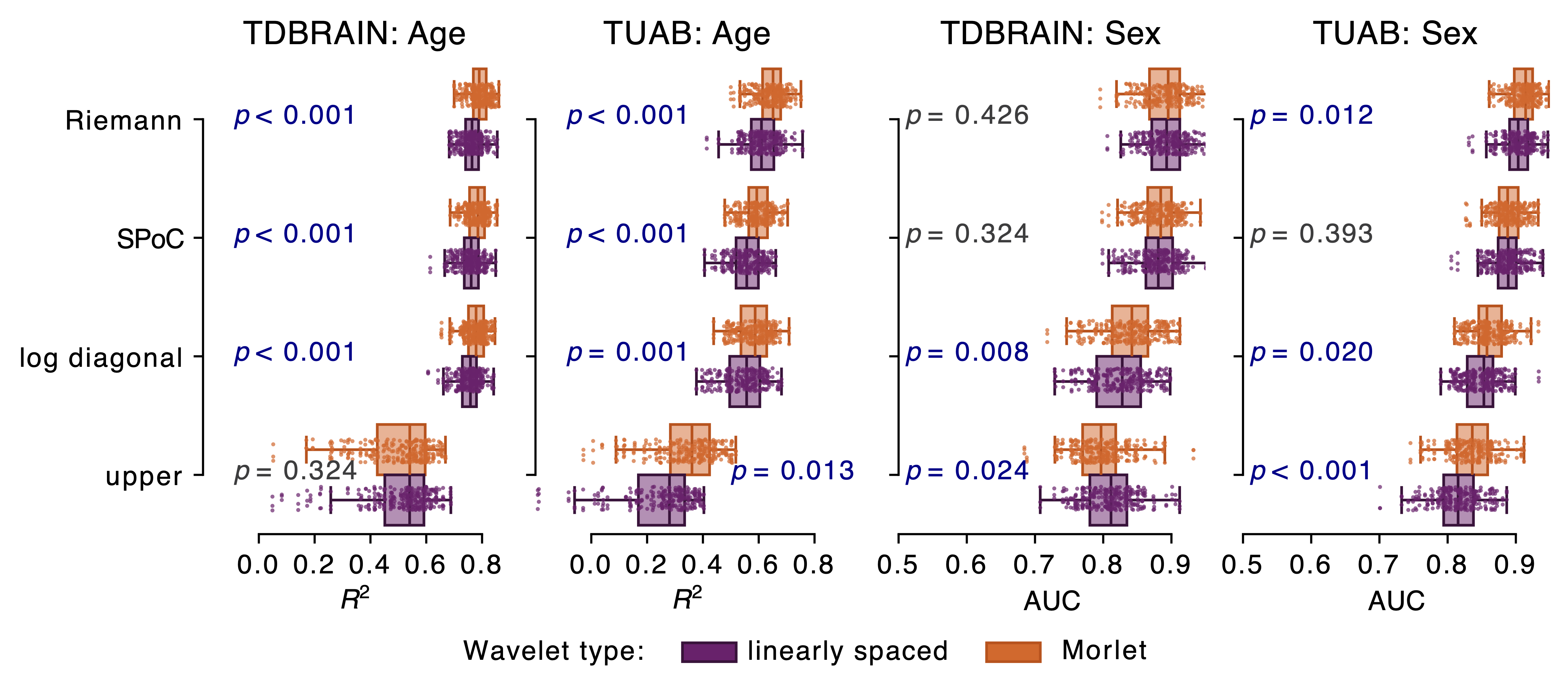
You may wonder by now, how our covariance-based models with Morlet wavelets compare to previous versions using bandpass filtering in conventional frequency bands. We did not have a strong desired outcome here but loosely conjectured that continuous frequencies with log-linear smoothing via Morlet wavelet-families might provide a good prior for capturing the frequency-specific smoothness of brain rhythms. We see in practice (Figure 8 a) that decoding with Morlet wavelets most of the time was leading to improved performance! And the sensitivity analysis in figure (Figure 8 b) shows that this is not trivially driven by the increased number of frequencies coming with the wavelet approach.
Thanks to one unknown reviewer, we even went the extra mile to see if this comes from the wavelet design itself (complex Gabor wavelet) or if it comes from logarithmic frequency placing and smoothing that defines Morlet wavelet families. To investigate this point, we computed another wavelet family with a linear frequency grid (hence no log-linear smoothing). Indeed, corroborating our initial intuition, the log-linear smoothing that comes with Morlet wavelets significantly improves performance (most of the time)!
Open-source software library and research code
One more thing. If you want to check out our wavelet pipeline and wish to deep dive into Morlet Wavelets, we’ve got you covered. Checkout meeglet – our Python and MATLAB package for doing M/EEG analysis using Morlet wavelets: https://roche.github.io/neuro-meeglet/
You also find our research code in case you wish to use the preprocessing pipelines and models from the paper for your own work: https://github.com/Roche/neuro-meeglet-paper
Thank you and looking forward
That was it! We hope this can inspire you to develop novel brain-specific EEG biomarkers or novel #ML methods that internally handle artifact isolation and suppression. Big shout out to the team: Philipp Bomatter, Joseph Paillard, Pilar Garces & Jörg Hipp!
Citation
@article{bomatter2024,
author = {Bomatter, Philipp and Paillard, Joseph and Garces, Pilar and Hipp, J{\"o}rg and Engemann, Denis-Alexander},
title = {Machine learning of brain-specific biomarkers from EEG},
year = {2024},
journal = {eBioMedicine},
url = {https://doi.org/10.1016/j.ebiom.2024.105259},
date = {2024/08/05},
publisher = {Elsevier},
isbn = {2352-3964},
month = {2024/08/06},
volume = {106},
}